Final Project Part 1: Lightfield Camera Project (Scroll down for part 2)

CS180: Intro to Computer Vision and Computational Photography

Lightfield Cameras

This project explores light field camera techniques by manipulating a grid of images taken along a single axis, demonstrating how shifting and averaging multiple images can simulate complex camera effects like depth refocusing and aperture adjustment. By capturing light rays from different perspectives, the project allows computational reconstruction of focus and aperture characteristics, revealing how simple mathematical operations can create sophisticated visual transformations that mimic advanced camera capabilities.

Depth Refocusing

Depth refocusing is a computational photography technique that exploits the parallax effect, where light rays from different points in a scene arrive at slightly different angles when the camera moves. By capturing a grid of images along a single axis, the technique captures how light rays from objects at different distances shift relative to each other, creating a unique depth-dependent positioning effect. The method centers on a reference image and shifts surrounding images using a scaling factor (alpha), which mathematically adjusts the trajectories of these light rays to simulate different focal planes. As nearby objects cause more significant light ray displacement compared to distant objects, the shifting and averaging process creates images that can selectively sharpen or blur different depth regions. By using alpha values ranging from -1 to 3, the technique manipulates these light ray intersections, effectively allowing computational reconstruction of focus at various depths without physically changing the camera's lens.

Depth Refocusing Gif (CLICK TO RESTART GIF)

Depth Refocusing

Aperture Adjustment

Aperture adjustment is a computational photography technique that simulates different camera aperture sizes by strategically selecting and averaging images from a light field grid. The implementation uses a radius-based approach to gradually reduce the number of images used in averaging, effectively mimicking how a smaller aperture would narrow the light gathering area of a camera. By selecting images from a central region of the grid and progressively reducing this region (from a radius of 0 to 7), the method creates a series of images that demonstrate how the apparent aperture size affects image sharpness and light gathering, without physically changing a camera lens. The code iterates through different radii, averaging only the images within that radius around a central reference point, which creates a computational representation of aperture adjustment that showcases how fewer light rays contribute to the final image. This technique allows for exploring depth of field and light gathering characteristics through simple mathematical operations on a grid of images taken from slightly different perspectives.

Depth Refocusing Gif (CLICK TO RESTART GIF)

Depth Refocusing

Summary

In this project, I learned that light field photography allows me to computationally manipulate images captured from multiple perspectives to simulate advanced camera techniques like depth refocusing and aperture adjustment without physically changing lens properties. By understanding how light rays from different scene depths shift across a grid of images, I discovered that simple mathematical operations like shifting and averaging can dramatically transform image characteristics, effectively reconstructing focus and depth information. I learned that the parallax effect—where nearby objects move more significantly across images compared to distant objects—can be leveraged to create computational photography effects that mimic complex optical systems. The project showed me that a grid of images captures not just a single moment, but a rich, multidimensional representation of light rays passing through different points in space, allowing for post-capture manipulation of visual properties. Most importantly, I gained insight into how computational techniques can deconstruct and reconstruct visual information by treating images as data to be mathematically transformed, revealing the underlying computational principles that make advanced imaging techniques possible.

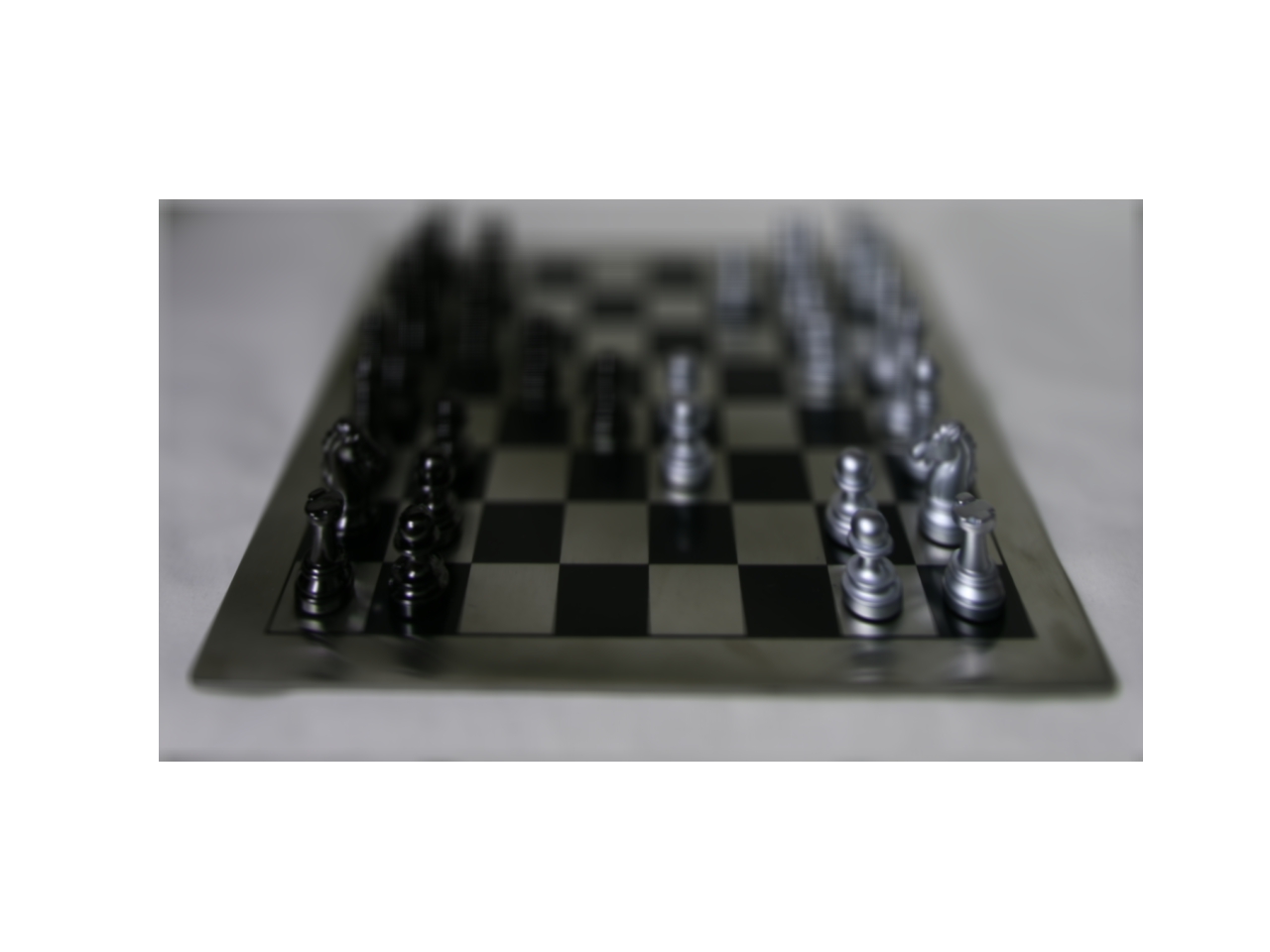
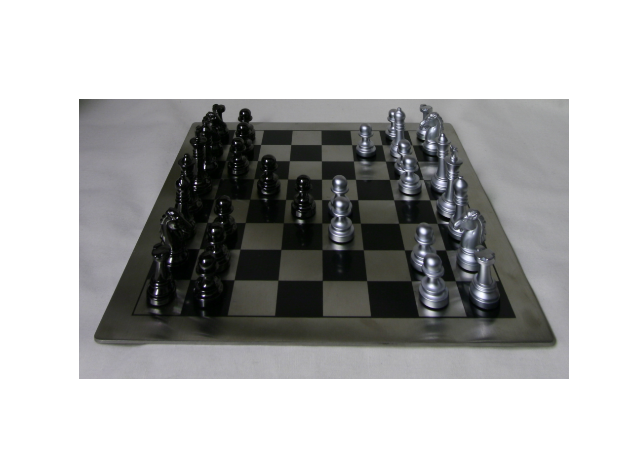
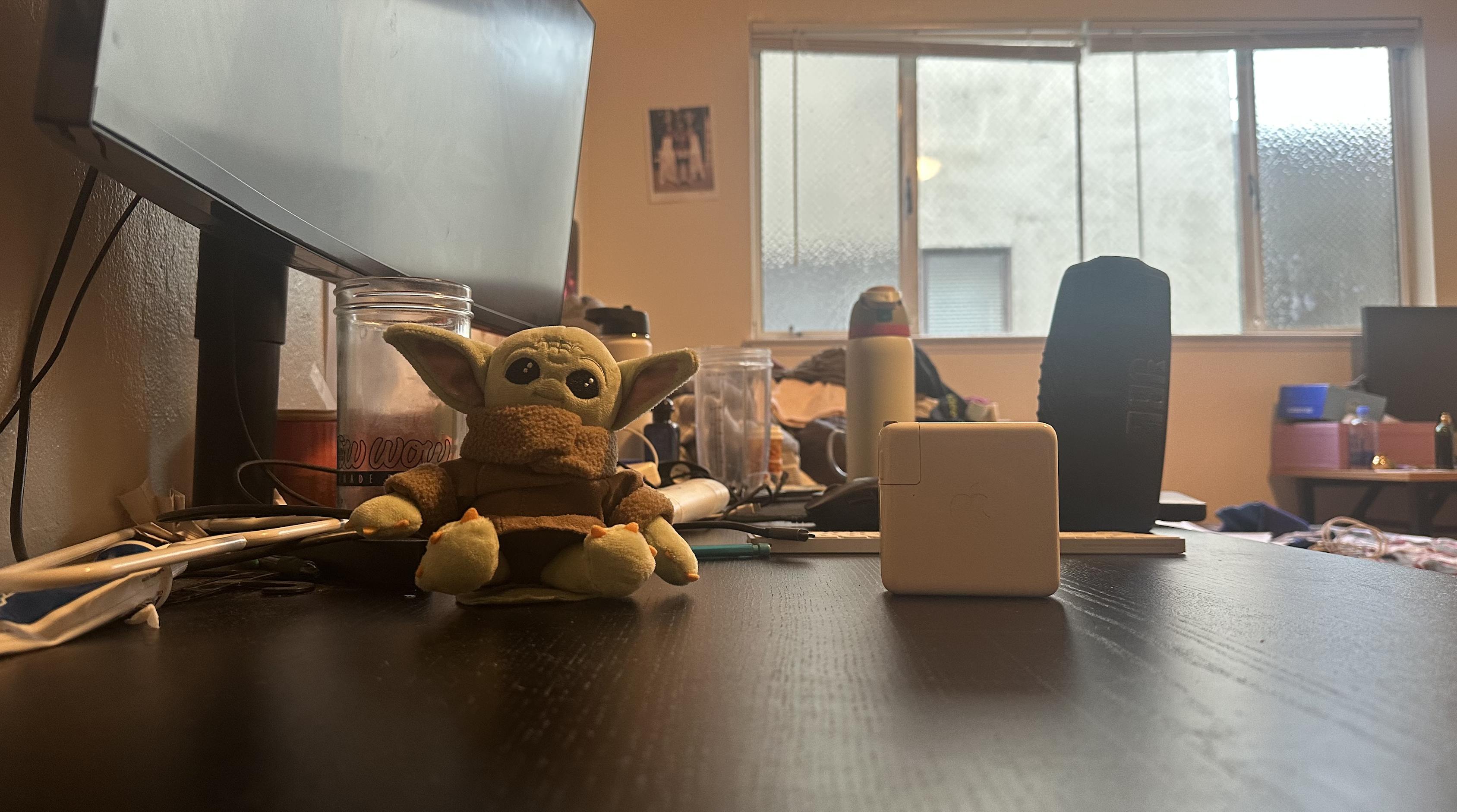
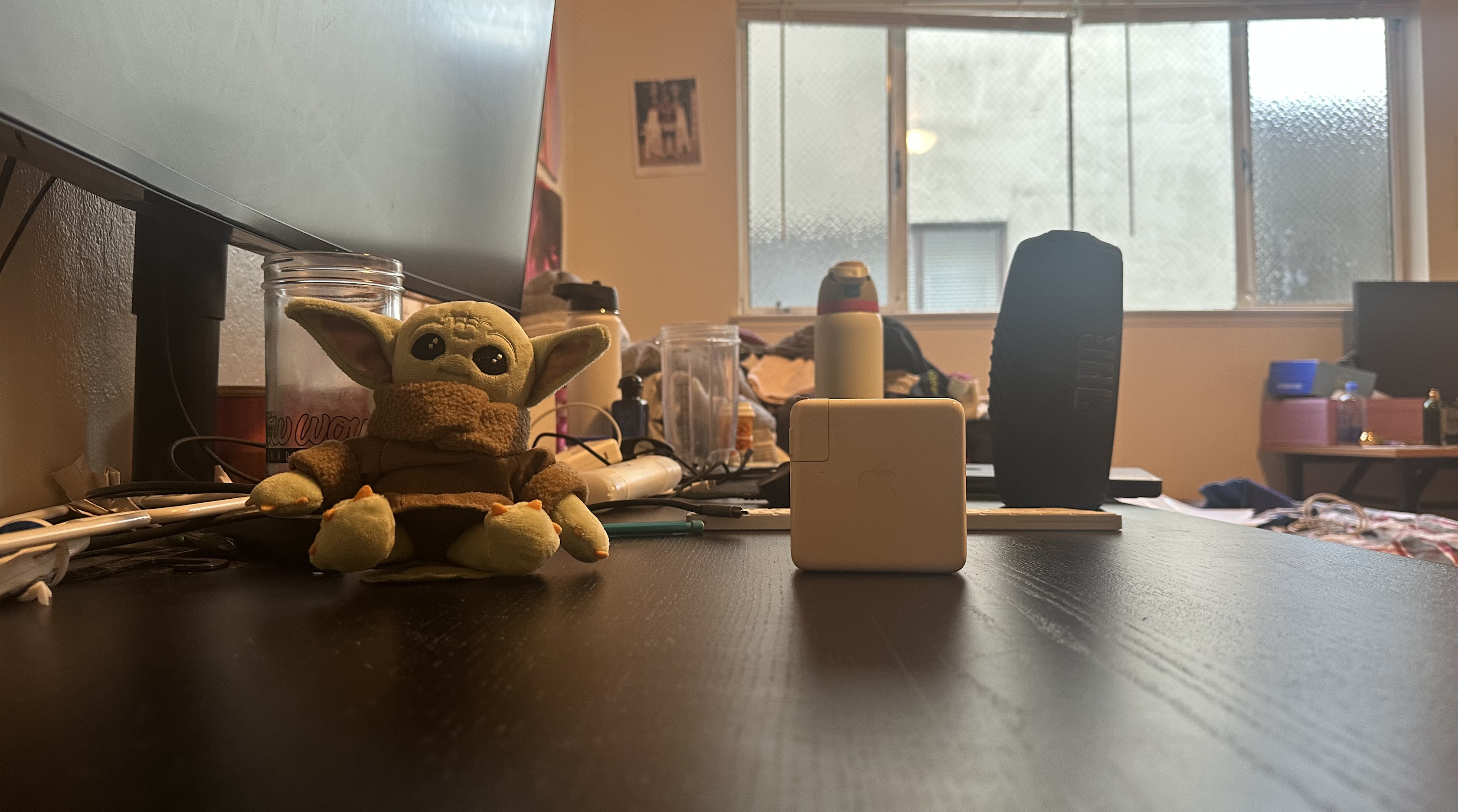
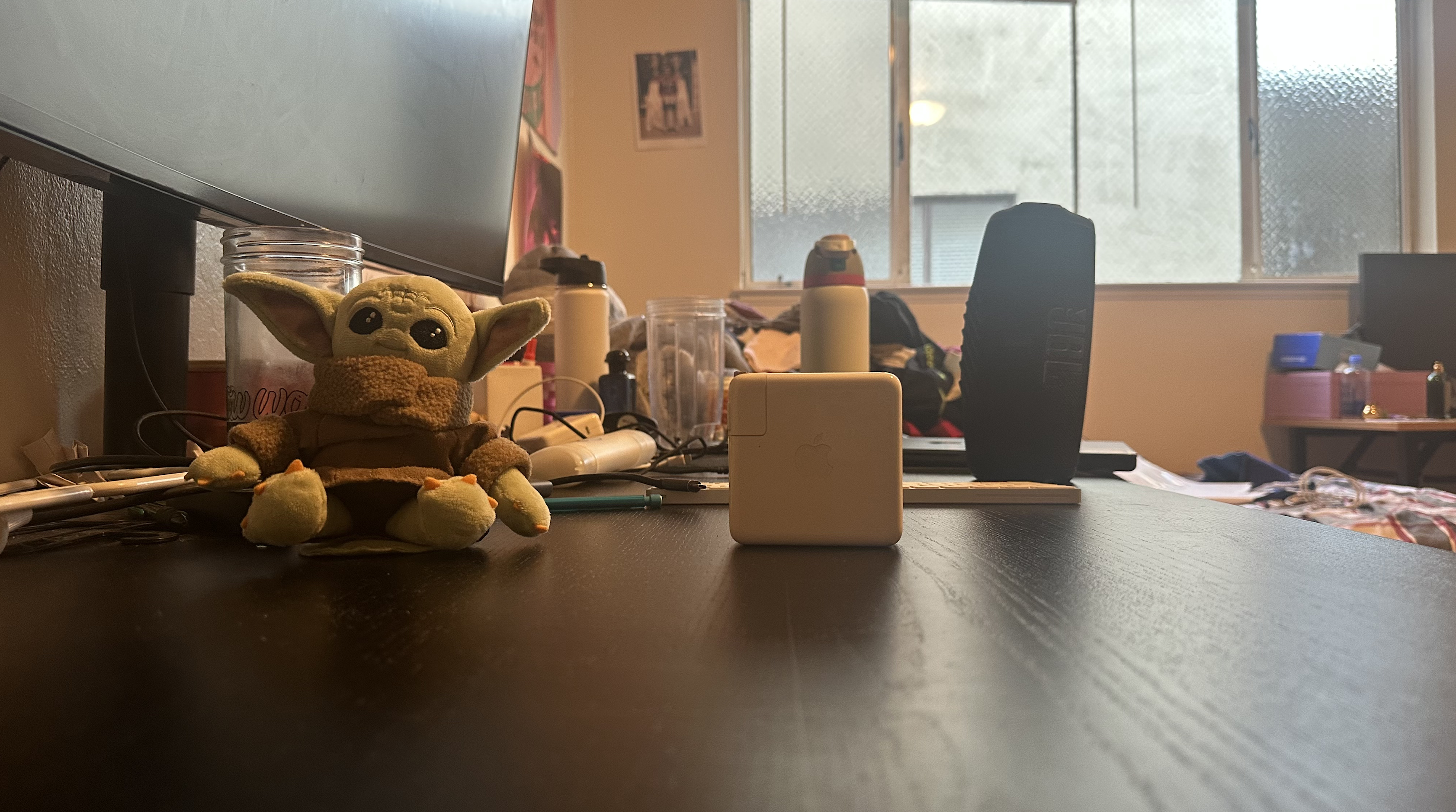
Bells and Whistles: Using Real Data

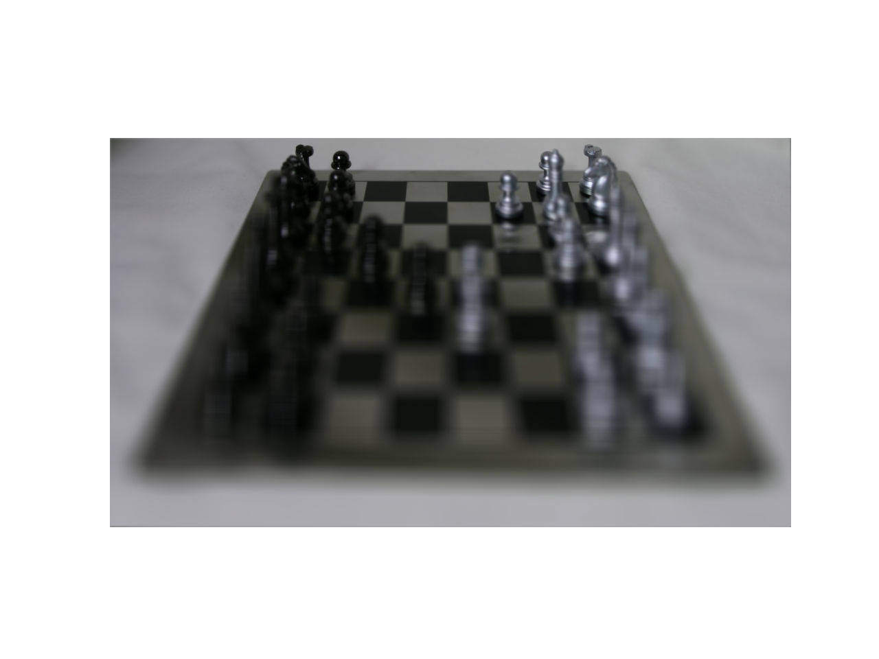
In this part, I took my own pictures to simulate a light field camera. I drew a 5x5 grid on my desk, drawing spaces 2.5 inches apart. My results for depth refocusing and aperture adjustment were quite blurry. I imagine this is due to the lack of precision in exact grid positions and angles for the effects to be successful. I also only had a 5x5 grid, which may not be large enough.

Depth Refocusing (CLICK TO RESTART GIF)

Depth Refocusing

Aperture Adjustment (CLICK TO RESTART GIF)

Aperture Refocusing

Final Project Part 2: HDR (High Dynamic Range) Images

CS180: Intro to Computer Vision and Computational Photography

High Dynamic Range

This project explores High Dynamic Range (HDR) imaging by developing computational techniques to combine multiple images with different exposures into a single radiance map that captures a broader range of light intensities than a single photograph can achieve. By recovering the camera's response curve, constructing a radiance map, and then applying sophisticated tone mapping techniques like bilateral filtering, the project demonstrates how computational photography can overcome the limitations of traditional camera sensors to create images that more accurately represent the visual complexity of real-world scenes.

Constructing the HDR Radiance Map

These graphs illustrate the key concepts behind the construction of an HDR radiance map from multiple exposure images. The first two graphs show the recovered camera response function g, which maps pixel values to the logarithm of scene radiance. The process involves solving a linear system that relates the observed pixel values, exposure times, and an unknown but smooth function g. The third graph plots the final HDR radiance values as a function of the log exposure, demonstrating the wide dynamic range that can be captured by combining multiple exposures. The final graph overlays the individual camera response curves, highlighting how each exposure contributes information about a different range of radiance values. Together, these visualizations reveal the computational steps required to extract the underlying radiance information from a set of differently exposed images. By recovering the nonlinear camera response and then combining the exposure-dependent pixel values, the HDR reconstruction process can faithfully represent the full luminance range of the original scene, going beyond the limited dynamic range of any single photograph.

G Curves
Left Image

First, the camera's response function, which maps pixel values to scene radiance, needs to be recovered. This is done by solving a linear system that relates the observed pixel values, exposure times, and an unknown but smooth function called g. The resulting g function essentially allows translating the pixel data from each image into a common scale of scene radiance. Next, the multiple exposure images are processed one by one. For each image, the pixel values are weighted based on how well-exposed they are - pixels that are too bright or too dark get lower weights, while mid-range pixels get higher weights. These weighted pixel values, along with the exposure time, are then used to compute contributions to two running totals - a numerator and a denominator. After processing all the input images, the final HDR radiance map is computed by dividing the numerator by the denominator on a per-pixel basis. This has the effect of combining the information from the different exposures into a single high dynamic range representation of the scene's luminance levels. The last step is to exponentiate this log-scaled radiance map to obtain the actual HDR radiance values. This final HDR radiance map can then be used for various downstream applications, such as tone mapping to generate a displayable image. The key advantage of this approach is that it allows capturing a much wider range of luminance values than any single photograph could, by intelligently fusing the limited dynamic range of multiple exposures. This is a powerful computational photography technique for overcoming the limitations of traditional camera sensors.

HDR Radiance Map
Depth Refocusing

Tone Mapping

The three tone-mapping methods presented—Global Scale, Global Simple, and Durand—represent different approaches to converting a high dynamic range (HDR) radiance map into a displayable image. HDR images capture a wider range of light intensities than typical images, but they require tone mapping to compress this range into values suitable for standard displays. Global Scale: This method linearly scales the pixel intensities in the HDR map based on the global minimum and maximum values. It's simple but often fails to preserve details in very dark or bright areas, leading to loss of contrast. Global Simple: Inspired by Reinhard et al., this approach compresses pixel intensities by dividing them by 1 + intensity. It maintains better overall contrast than Global Scale, producing more balanced results, especially in areas with extreme brightness. Durand: This method uses a local tone mapping technique, applying a bilateral filter to separate the HDR image into base (large-scale) and detail layers. It compresses the dynamic range of the base layer while preserving local details and recombines them with chrominance for more nuanced and realistic results.

Tone Mapping Results
Right Image