Project Description
The goal of this project is to explore image warping and mosaicing. We take multiple photographs, align them using homographies, warp them, and blend them into a mosaic. The project introduces concepts of projective transformations and teaches how to compute homographies and use them for image mosaicing.
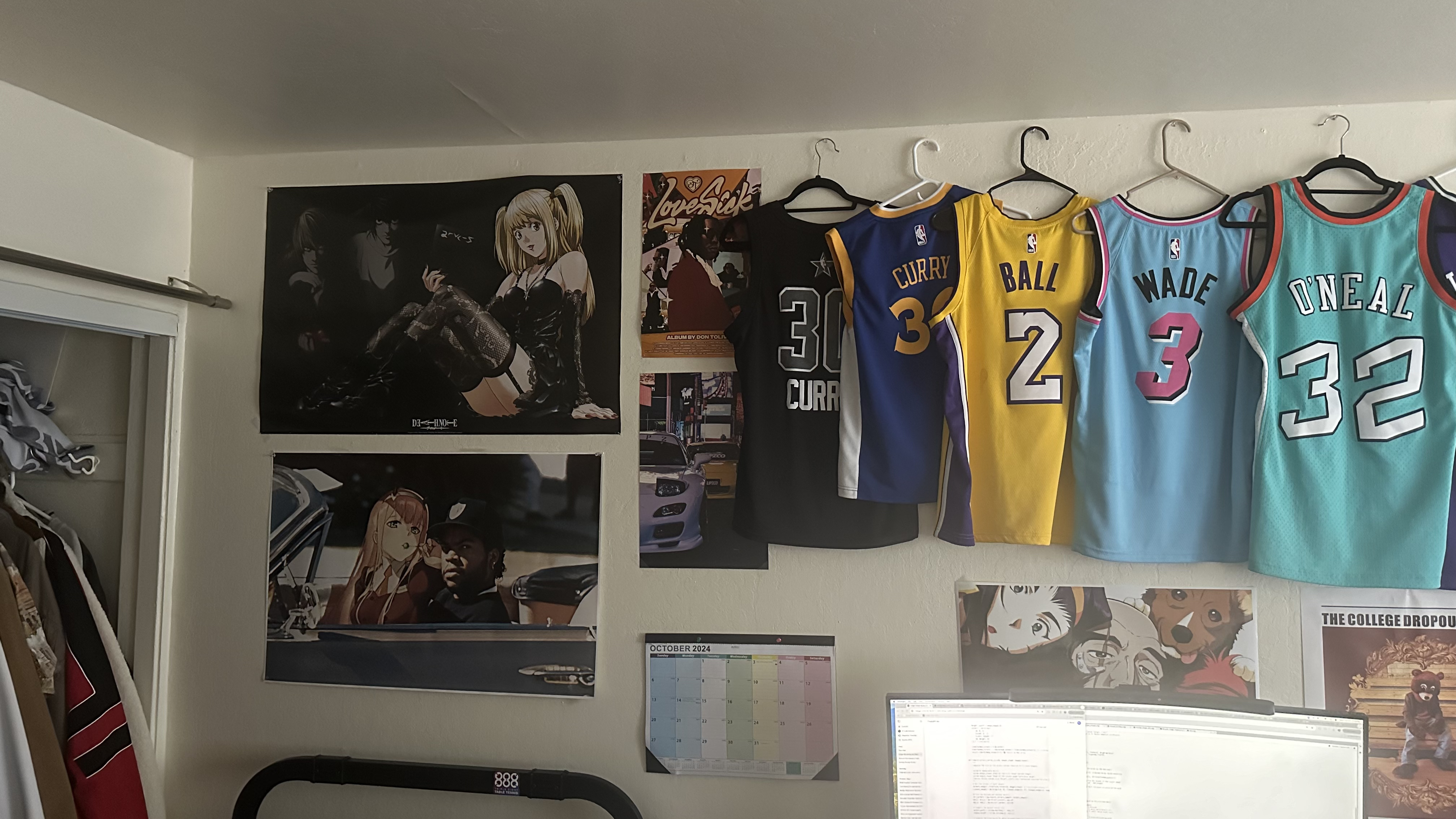
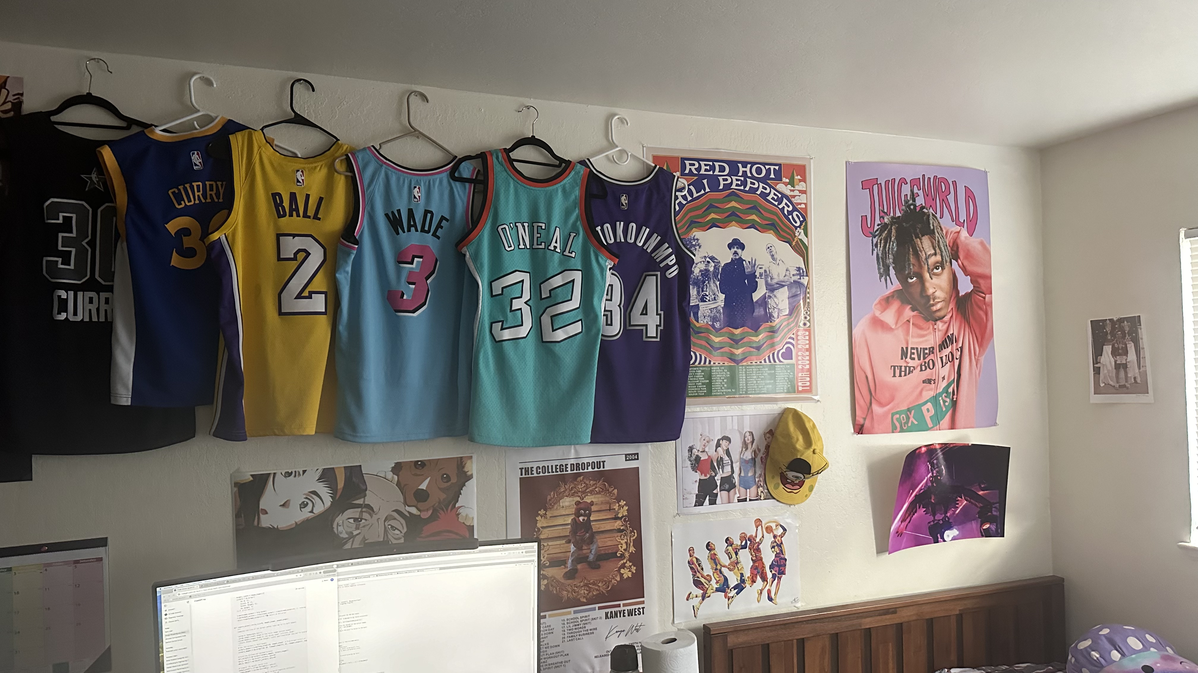
Shoot the Pictures
(Description of the process, leaving space for images)
Recover Homographies
Homography Process
A homography is a transformation between two images that describes how points in one image correspond to points in another, based on a projective transformation. The homography matrix H is a 3x3 matrix that maps a point p in one image to its corresponding point p' in another image, using the equation:
p' = H * p
Here, p and p' are points in homogeneous coordinates, which means they are represented as 3D vectors [x, y, 1]. The homography matrix H has eight degrees of freedom and is typically expressed as:
                    H = | h11  h12  h13 |
                        | h21  h22  h23 |
                        | h31  h32  h33 |
To compute H, we need at least 4 pairs of corresponding points between two images. Each point correspondence gives two equations, and with four point pairs, we have enough equations to solve for the 8 unknowns (the ninth value is set to 1 for normalization). The system of equations is solved using methods like Singular Value Decomposition (SVD).
Once the homography matrix is computed, we can apply it to map every pixel in one image to its corresponding location in the second image, enabling us to warp one image into the perspective of the other.
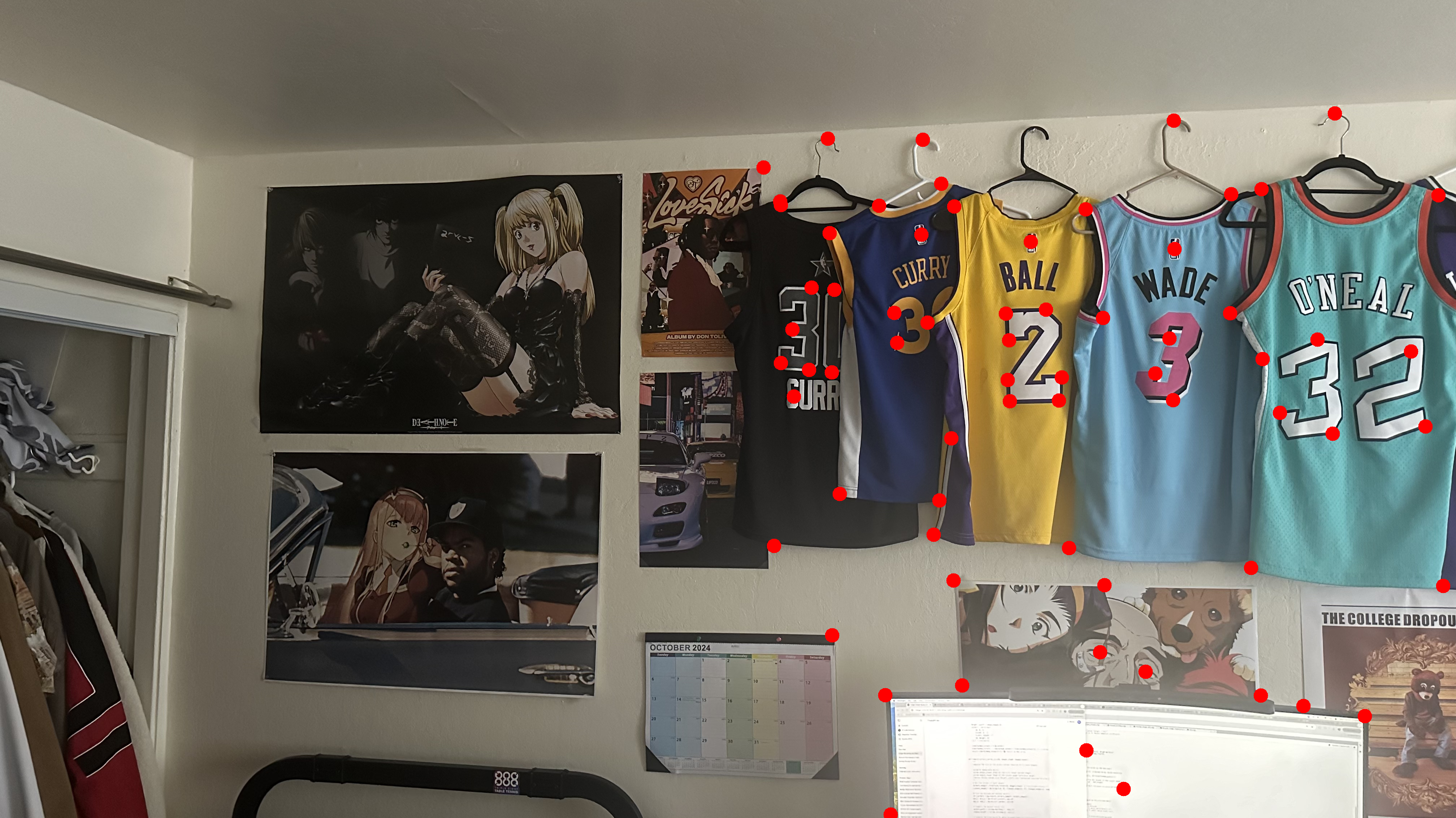
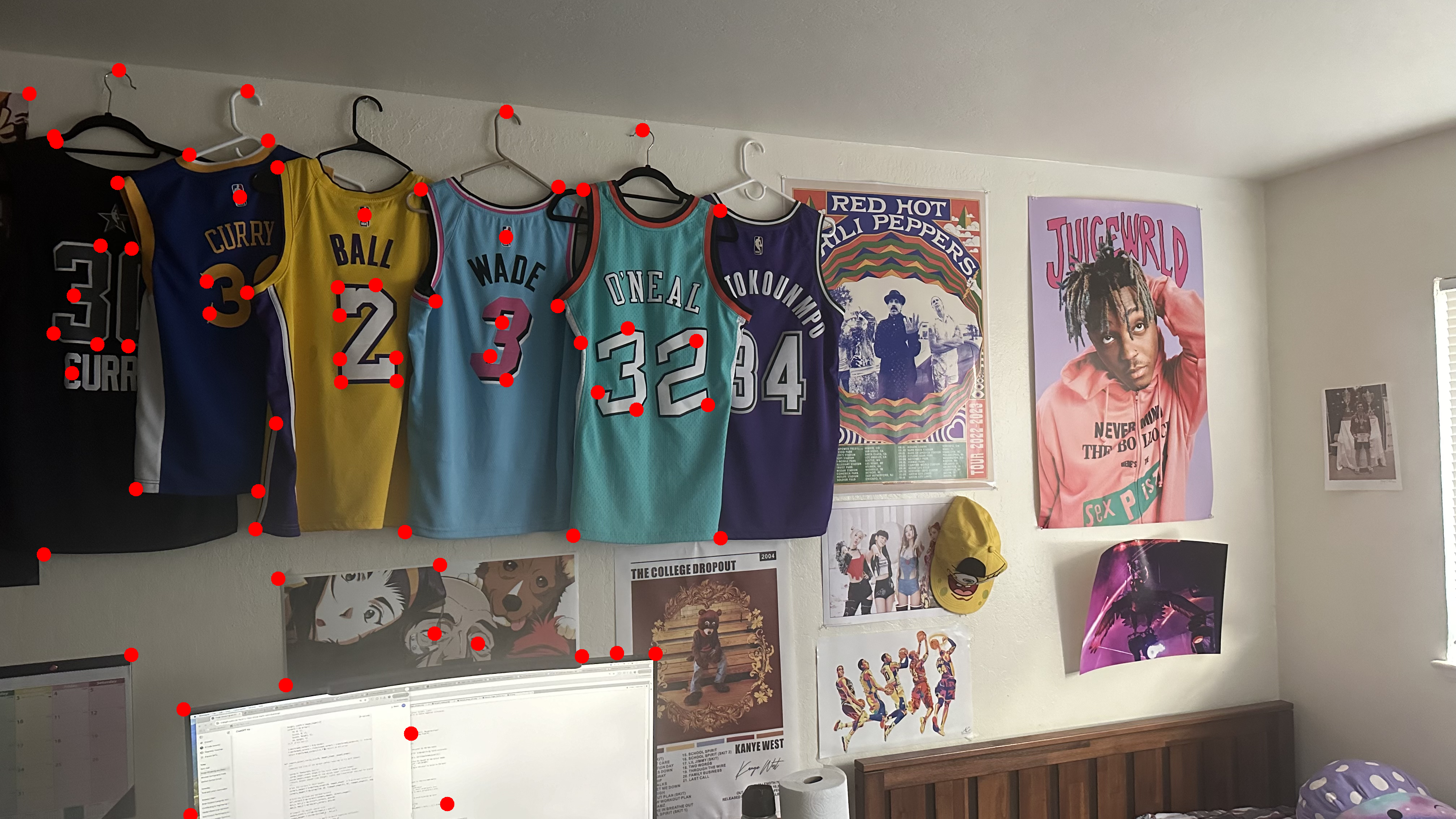
Image Warping Process
The warping process aligns one image to the perspective of another using a homography matrix, which defines how points in one image map to corresponding points in another. The homography is a 3x3 matrix that accounts for transformations such as translation, rotation, scaling, and perspective changes.
To apply the homography, each pixel in the source image is transformed to new coordinates in the target image. This is known as forward warping. In this project, the left image is warped to match the right image by calculating where each pixel from the left image should appear in the final mosaic.
A translation matrix is also applied to ensure that all parts of the warped image fit within the output canvas, preventing any negative or out-of-bounds pixel coordinates. The warped image is then placed into this larger canvas, aligning it with the reference image.
The result is a transformed version of the left image, reprojected onto the same plane as the right image, ready for blending into a mosaic.
Blending and Mosaicing Process
In this project, images are blended into a mosaic using weighted averaging to ensure smooth transitions in overlapping regions. First, the left image is warped into the perspective of the right image using a homography matrix. To blend them, we create alpha masks for both images, indicating valid pixels. These masks are then used to compute blend masks that determine the contribution of each image in the overlapping areas.
The weighted averaging formula for each image is:
                blend_mask1 = mask1 / (mask1 + mask2 + ϵ),
                blend_mask2 = mask2 / (mask1 + mask2 + ϵ)
This ensures that pixels are mixed smoothly based on their mask values. In the final step, the pixel values from both images are combined using these blend masks, resulting in a seamless mosaic where edges between the images are blurred and integrated naturally. This avoids harsh transitions and creates a coherent panoramic view.
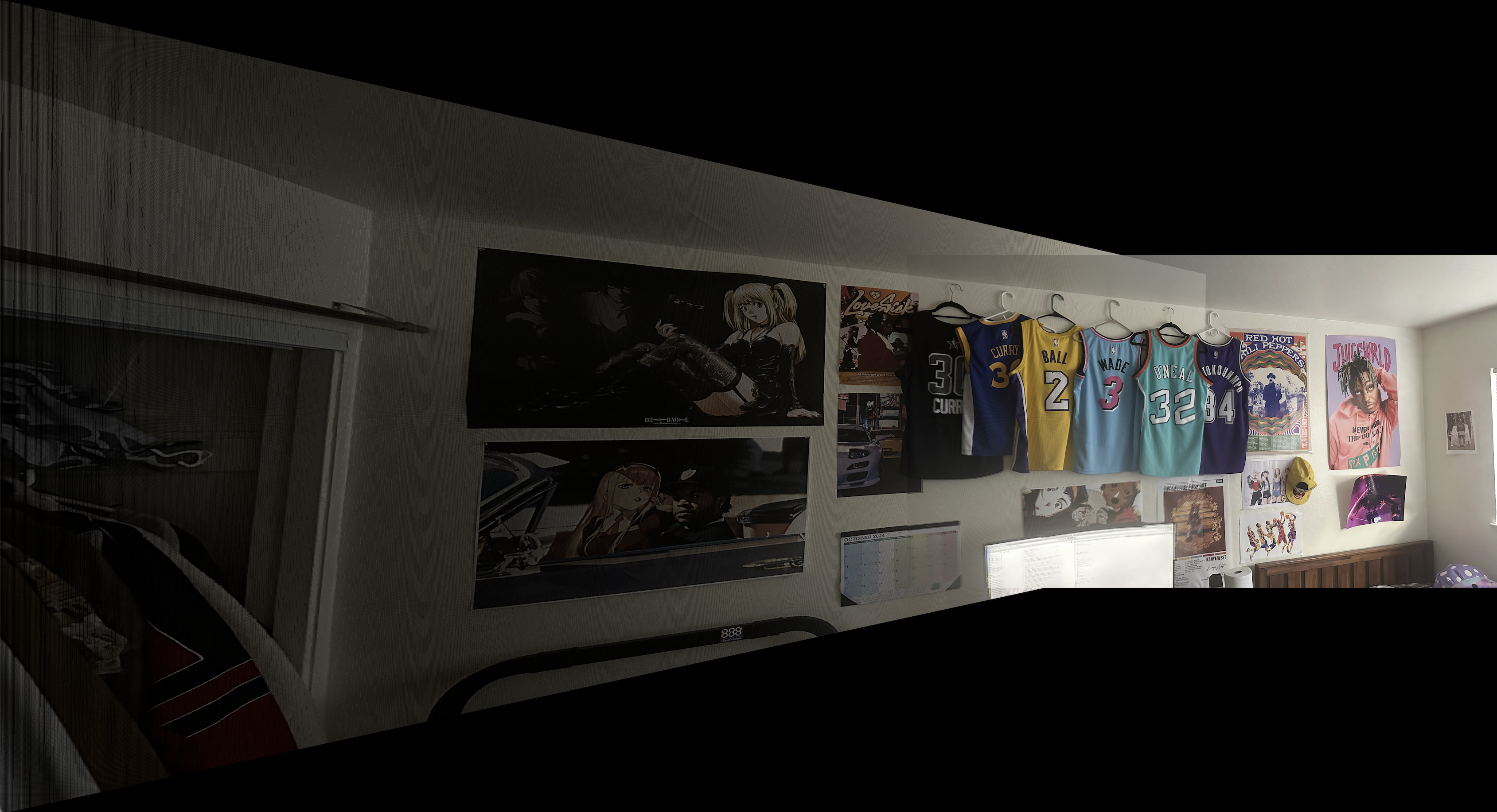
Image Rectification
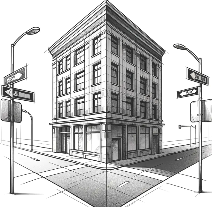
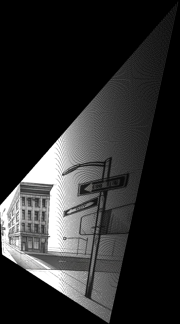
Image rectification is the process of transforming an image so that a certain planar surface appears front-facing and rectangular. We achieve this by computing a homography based on known correspondences. In this case, we take an image of a building from a perspective. Then I create correspondence points for the 4 corners of the right plane of this building. We will transform this into a front facing, rectangular surface and visualize the final result of the image when this is done. In this case, I transformed this into size 100,200 as this seems to be the approximate ratio of that face in the original image. You might notice that the final result does not have a perfect rectangle. This is because it is very sensitive to the correspondence points not representing the perfect corners of the rectangle in the original building. I was not able to get perfect points because there is noise in selecting points on an image manually.
Below is an example of image rectification:
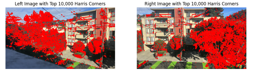
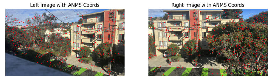
Feature Matching for Autostitching
Using the harris interest point detector, corners of interest are selected based on directional gradients and thresholded for the final corner set.
Adaptive Non-Maximal Suppression
Because there are too many Harris corners to efficiently compute, we use adaptive non maximal suppression to eliminate some corners. This approach involves iterating over each corner and identifying the nearest corner that has a significantly larger value, defined by the condition \( x_i < c_{\text{robustness}} \times x_j \), where \( x_i \) is the current corner, \( x_j \) represents all other corners, and \( c_{\text{robustness}} \) is set to 0.9. Next, the corners with the greatest distance to another corner meeting this threshold are selected. I set the number of selected corners to 500.
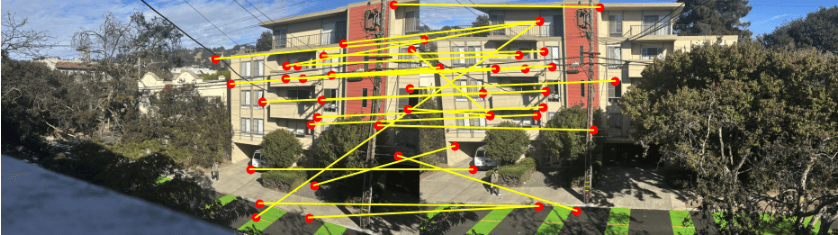
Feature Matching
To filter matching corners, a feature matching technique is applied. For each corner, a 40x40 patch is extracted from the image, centered on the corner point. This patch is resized to 8x8, normalized by subtracting the mean and dividing by the standard deviation to minimize intensity differences, and then flattened into a 1D feature vector. For each feature in image A, its error is calculated against all features in image B. Using Lowe’s ratio test, if the ratio of the two smallest errors is below a threshold of 0.5, the feature in image B with the smallest error is selected as the best match for the feature in image A.
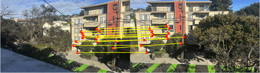
RANSAC
Unfortunately, some matches are still not very accurate as correspondence points. The reason I say not very accurate is because they cause large shifts in calculations of H, the homography matrix. RANSAC is an iterative process that tests homography matrices from subsets of points of all the matches by warping 4 points using the homography matrix, and then labeling those points who show accurate results as inliers. The threshold of how close warped points have to be to their computed match is a parameter, which I set to 5 pixels.
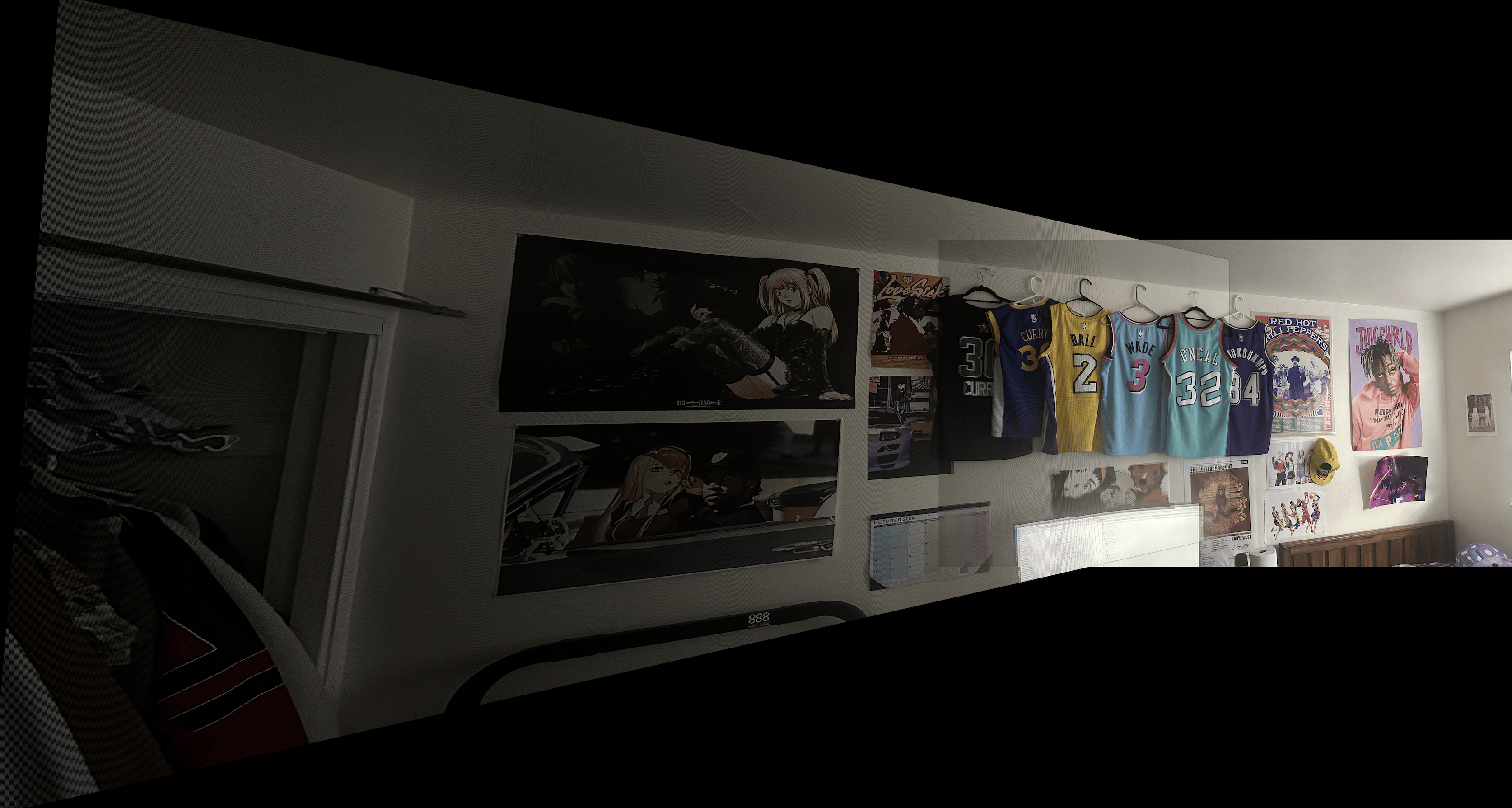
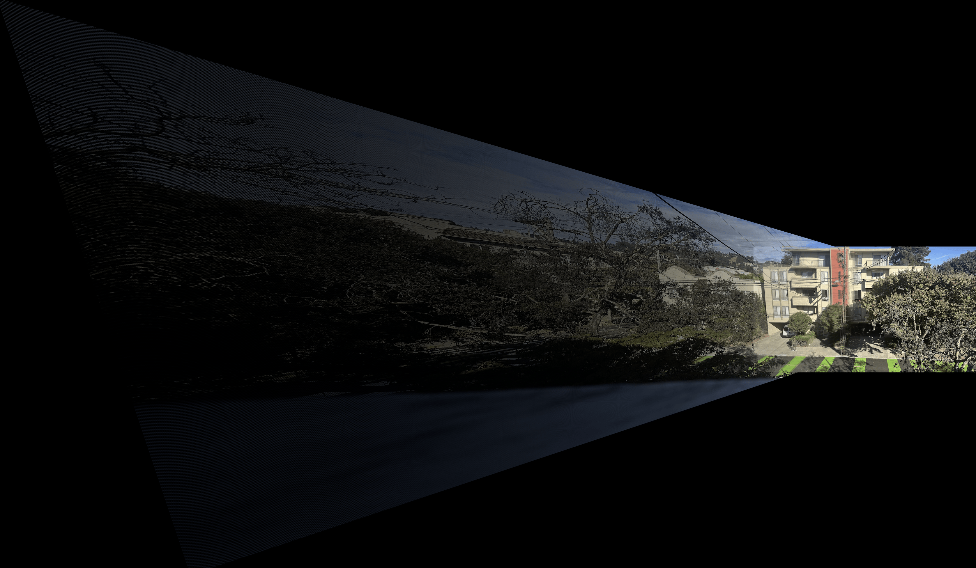
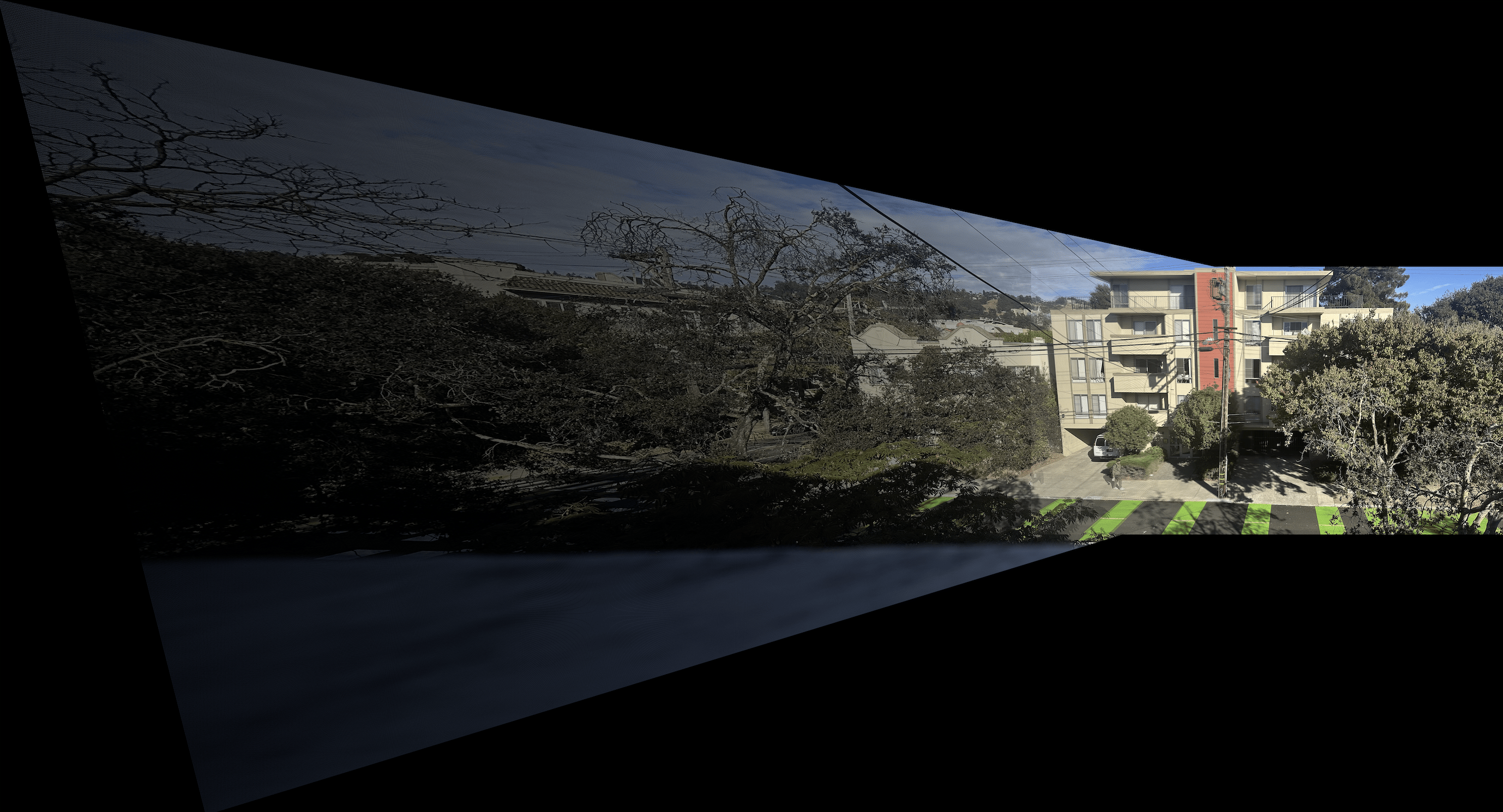
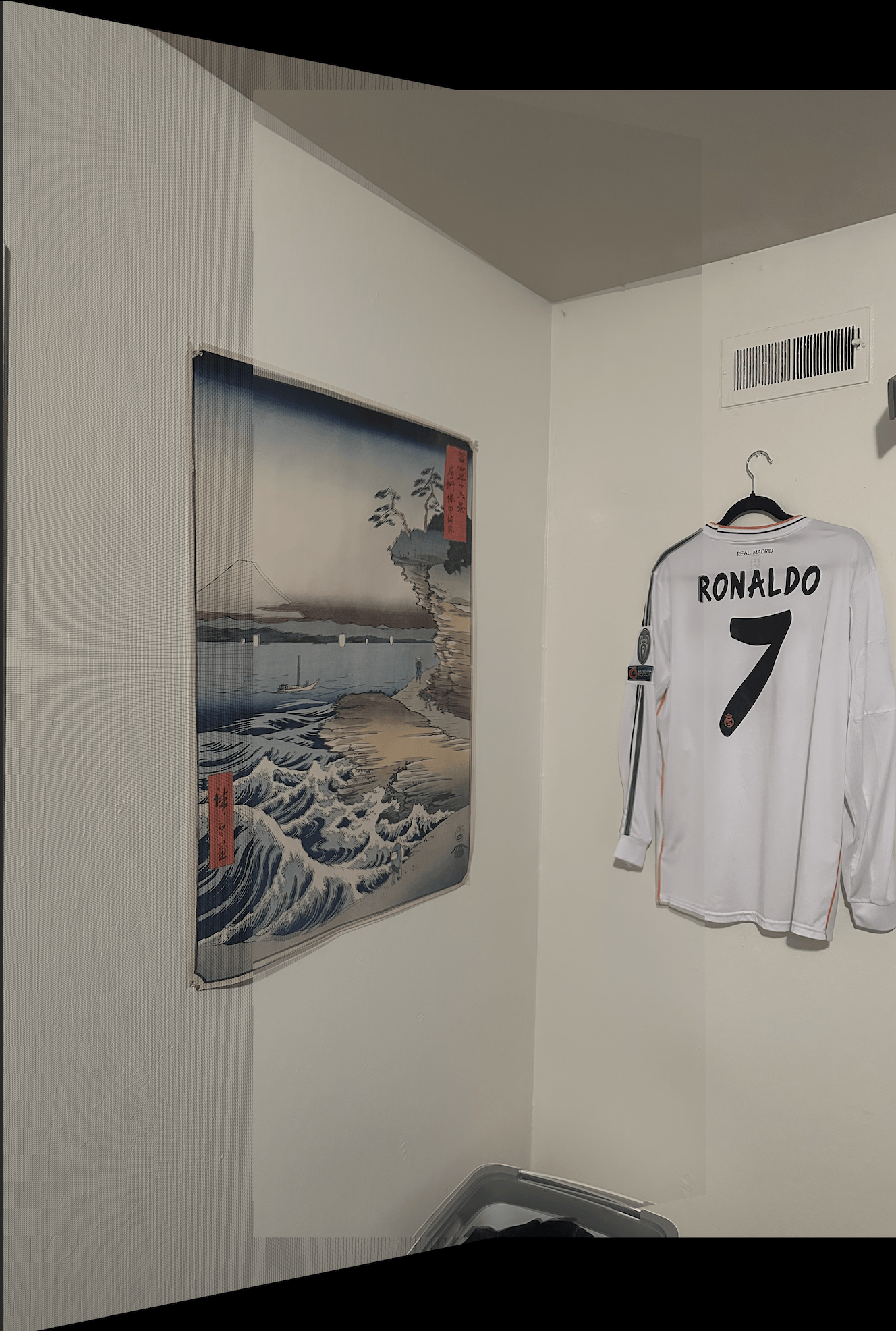
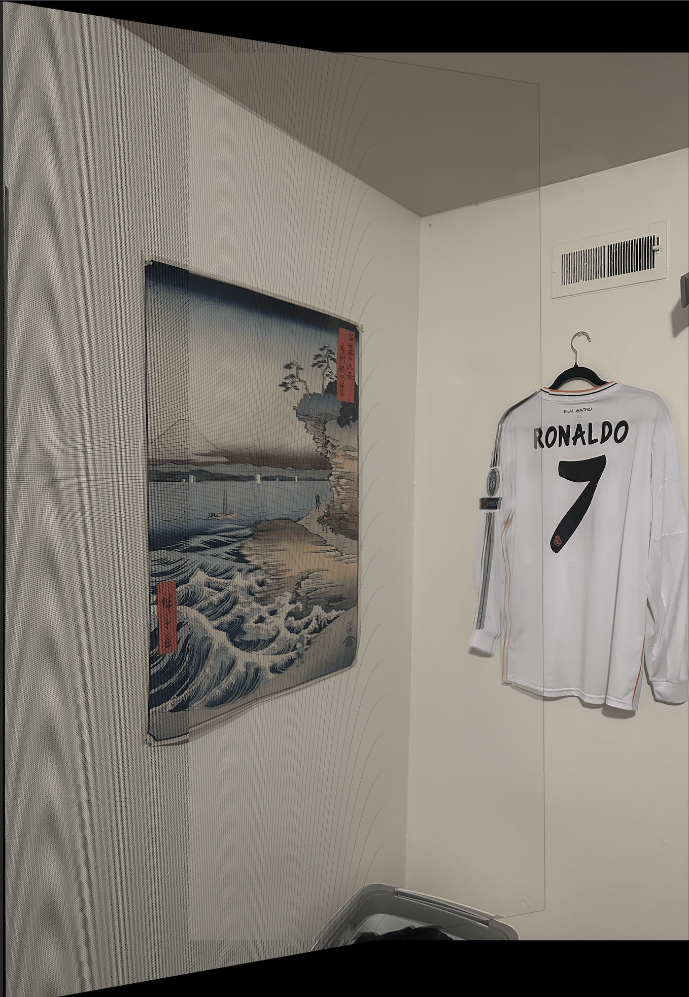
It seems that there are mixed results. For the balcony, you can see less blur in the orange area for the auto stitched mosaic, indicating better results. For the corner image, you can see a better computed homography as the images are more properly aligned. However, for the bedroom, it seems that the manual is actually better. The reason for this and also what was really my cool takeaway from this project is that it makes perfect sense that doing this process manually can actually lead to better results. Both of these methods are simply forms of picking corresponding points - the matching algorithms are the same. Since I spent a lot of time picking many correspondence points for the bedroom image manually, it actually turns out that this has a better result. However, it is without a doubt that the RANSAC auto stitching method using harris corners is superior when generalized to more complex situations. The efficiency to compute so many correspondence points is unmatched. Although using gradients may be less effective on an indivdual point scale, generalizing to thousands or millions of points requires something like harris plus RANSAC, since it is more efficient, and likely very accurate because the sample size is now huge and noise will often balance out.